Exploring Data with Pandas
We learned some of the ways pandas makes working with data easier than NumPy:
Axis values in dataframes can have string labels, not just numeric ones, which makes selecting data much easier.
Dataframes can contain columns with multiple data types: including integer, float, and string.
DataFrame.head() and DataFrame.info() methods
f500_head=f500.head()
f500.info()<class 'pandas.core.frame.DataFrame'>
Index: 500 entries, Walmart to AutoNation
Data columns (total 16 columns):
# Column Non-Null Count Dtype
--- ------ -------------- -----
0 rank 500 non-null int64
1 revenues 500 non-null int64
2 revenue_change 498 non-null float64
3 profits 499 non-null float64
4 assets 500 non-null int64
5 profit_change 436 non-null float64
6 ceo 500 non-null object
7 industry 500 non-null object
8 sector 500 non-null object
9 previous_rank 500 non-null int64
10 country 500 non-null object
11 hq_location 500 non-null object
12 website 500 non-null object
13 years_on_global_500_list 500 non-null int64
14 employees 500 non-null int64
15 total_stockholder_equity 500 non-null int64
dtypes: float64(3), int64(7), object(6)
memory usage: 66.4+ KBVectorized Operations
Because pandas is designed to operate like NumPy, a lot of concepts and methods from Numpy are supported. Recall that one of the ways NumPy makes working with data easier is with vectorized operations, or operations applied to multiple data points at once:
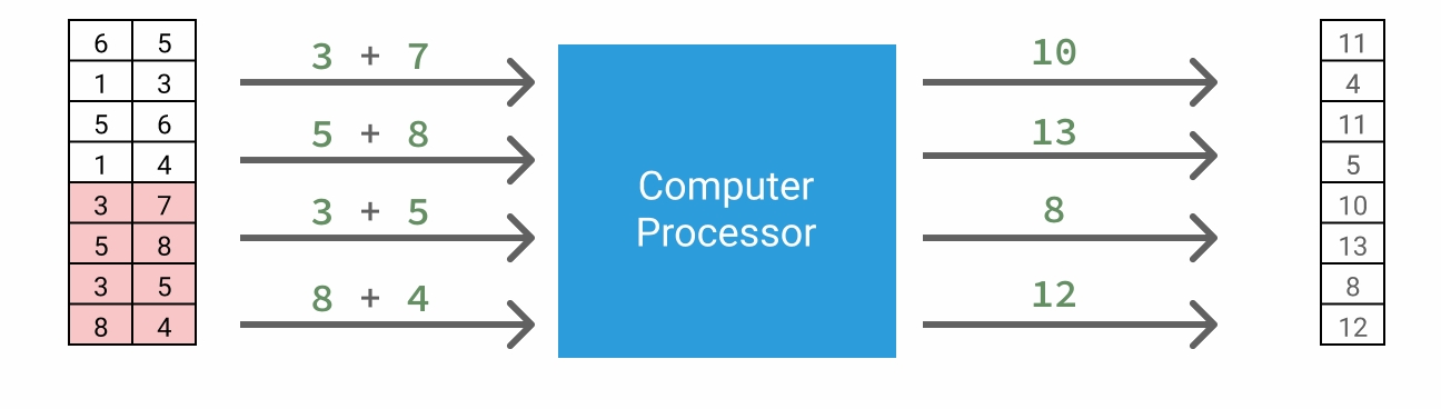
Vectorization not only improves our code's performance, but also enables us to write code more quickly.
Because pandas is an extension of NumPy, it also supports vectorized operations. Let's look at an example of how this would work with a pandas series:
Just like with NumPy, we can use any of the standard Python numeric operators with series, including:
series_a + series_b - Addition
series_a - series_b - Subtraction
series_a * series_b - Multiplication (this is unrelated to the multiplications used in linear algebra).
series_a / series_b - Division
Example
Let's use vectorized operations to calculate the changes in rank for each company. To achieve this, we'll subtract the current rank column from the previous_rank column. This determines whether a particular company moved upwards or downwards. A positive result indicates improved ranking, while a negative result indicates a drop in ranking. A zero result means the company retained its position.
Subtract the values in the rank column from the values in the previous_rank column. Assign the result to rank_change.
Below are the first five values of the result:
We can observe from the results that Sinopec Group and Toyota Motor each increased in rank from the previous year, while China National Petroleum dropped a spot. However, what if we wanted to find the biggest increase or decrease in rank?
Like NumPy, pandas supports many descriptive stats methods that can help us answer these questions. Here are a few of the most useful ones (with links to documentation):
Use the Series.max() method to find the maximum value for the rank_change series. Assign the result to the variable rank_change_max.
Use the Series.min() method to find the minimum value for the rank_change series. Assign the result to the variable rank_change_min.
we used the Series.max() and Series.min() methods to figure out the biggest increase and decrease in rank:
Biggest increase in rank: 226
Biggest decrease in rank: -500
However, according to the data dictionary, this list should only rank companies on a scale of 1 to 500. Even if the company ranked 1st in the previous year moved to 500th this year, the rank change calculated would be -499. This indicates that there is incorrect data in either the rank column or previous_rank column.
Next, we'll learn another method that can help us more quickly investigate this issue - the Series.describe() method. This method tells us how many non-null values are contained in the series, along with the mean, minimum, maximum, and other statistics
You may notice that the values in the code segment above look a little bit different. Because the values for this column are too long to neatly display, pandas has displayed them in E-notation, a type of scientific notation:
5.000000E+02
5.000000 * 10 ** 2
500
2.436323E+05
2.436323 * 10 ** 5
243632.3
Describe function
If we use describe() on a column that contains non-numeric values, we get some different statistics. Let's look at an example:
The first statistic, count, is the same as for numeric columns, showing us the number of non-null values. The other three statistics are new:
unique: Number of unique values in the series. In this case, it tells us that there are 34 different countries represented in the Fortune 500.
top: Most common value in the series. The USA is the country that headquarters the most Fortune 500 companies.
freq: Frequency of the most common value. Exactly 132 companies from the Fortune 500 are headquartered in the USA.
Return a series of descriptive statistics for the rank column in f500.
Select the rank column. Assign it to a variable named rank.
Use the Series.describe() method to return a series of statistics for rank. Assign the result to rank_desc.
Return a series of descriptive statistics for the previous_rank column in f500.
Select the previous_rank column. Assign it to a variable named prev_rank.
Use the Series.describe() method to return a series of statistics for prev_rank. Assign the result to prev_rank_desc.
When you reviewed the results you might have noticed something odd - the minimum value for the previous_rank column is 0.
However, this column should only have values between 1 and 500 (inclusive), so a value of 0 doesn't make sense. To investigate the possible cause of this issue, let's confirm the number of 0 values that appear in the previous_rank column.
Series.value_counts()
Let's use the Series.value_counts() method and Series.loc next to confirm the number of 0 values in the previous_rank column.
Use Series.value_counts() and Series.loc to return the number of companies with a value of 0 in the previous_rank column in the f500 dataframe. Assign the results to zero_previous_rank.
Dataframe Exploration Methods
In the last exercise, we confirmed that 33 companies in the dataframe have a value of 0 in the previous_rank column. Given that multiple companies have a 0 rank, we might (correctly) conclude that these companies didn't have a rank at all for the previous year. By definition, this means that the previous_rank for these companies is not a number! Therefore, it makes sense for us to replace these values with a NaN value instead of using a 0 to represent missing data. There are many advantages to doing this. A few of them are listed below:
Improved data analysis: By using NaN values to represent missing data, the rest of the data can still be analyzed and processed, allowing for a better understanding of the patterns and relationships in the data.
Improved readability: Datasets that use NaN values to represent missing data are more readable, as it clearly indicates the presence of missing values in the dataset.
Easy representation of missing data: By using NaN values, missing data in a dataset can be easily represented and identified, rather than using placeholder values such as 0 or -1 which can make interpreting results of calculations very difficult or misleading.
Before we correct these values, let's explore the rest of our dataframe to make sure there are no other data issues. Just like we used descriptive stats methods to explore individual series, we can also use descriptive stats methods to explore our f500 dataframe.
Because series and dataframes are two distinct objects, they have their own unique methods. However, there are many times where both series and dataframe objects have a method of the same name that behaves in similar ways. Below are some examples:
Unlike their series counterparts, dataframe methods require an axis parameter so we know which axis to calculate across. While you can use integers to refer to the first and second axis, pandas dataframe methods also accept the strings "index" and "columns" for the axis parameter:

For instance, if we wanted to find the median (middle) value for the revenues and profits columns, we could use the following code:
In fact, the default value for the axis parameter with these methods is axis=0. We could have just used the median() method without a parameter to get the same result!
Use the DataFrame.max() method to find the maximum value for only the numeric columns from f500 (you may need to check the documentation). Assign the result to the variable max_f500.
Dataframe Describe Method
Like series objects, dataframe objects also have a DataFrame.describe() method that we can use to explore the dataframe more quickly.
One difference is that we need to manually specify if you want to see the statistics for the non-numeric columns. By default, DataFrame.describe() will return statistics for only numeric columns. If we wanted to get just the object columns, we need to use the include=['O'] parameter:
count
500
500
500
500
500
500
unique
500
58
21
34
235
500
top
D. James Umpleby III
Banks: Commercial and Savings
Financials
USA
Beijing, China
http://www.conocophillips.com
freq
1
51
118
132
56
1
Keep in mind that whereas the Series.describe() method returns a series object, the DataFrame.describe() method returns a dataframe object. Let's practice using the dataframe describe method next.
Return a dataframe of descriptive statistics for all of the numeric columns in f500. Assign the result to f500_desc.
Assignment with pandas
After reviewing the descriptive statistics for the numeric columns in f500, we can conclude that no values look unusual besides the 0 values in the previous_rank column. Previously, we concluded that companies with a rank of zero didn't have a rank at all. Next, we'll replace these values with a null value to clearly indicate that the value is missing.
We'll learn how to do two things so we can correct these values:
Perform assignment in pandas.
Use boolean indexing in pandas.
Let's start by learning assignment, starting with the following example:
Just like in NumPy, the same techniques that we use to select data could be used for assignment. When we selected a whole column by label and used assignment, we assigned the value to every item in that column.
By providing labels for both axes, we can assign them to a single value within our dataframe.
The company "Dow Chemical" has named a new CEO. Update the value where the row label is Dow Chemical and for the ceo column to Jim Fitterling in the f500 dataframe
Using Boolean Indexing with pandas Objects
Now that we know how to assign values in pandas, we're one step closer to correcting the 0 values in the previous_rank column.
While it's helpful to be able to replace specific values when we know the row label ahead of time, this can be cumbersome when we need to replace many values. Instead, we can use boolean indexing to change all rows that meet the same criteria, just like we did with NumPy.
Let's look at two examples of how boolean indexing works in pandas. For our example, we'll work with this dataframe of people and their favorite numbers:

Let's check which people have a favorite number of 8. First, we perform a vectorized boolean operation that produces a boolean series:

We can use that series to index the whole dataframe, leaving us with the rows that correspond only to people whose favorite number is 8:

Note that we didn't use loc[]. This is because boolean arrays use the same shortcut as slices to select along the index axis. We can also use the boolean series to index just one column of the dataframe:

In this case, we used df.loc[] to specify both axes.
Next, let's use boolean indexing to identify companies belonging to the "Motor Vehicles and Parts" industry in our Fortune 500 dataset.
Create a boolean series, motor_bool, that compares whether the values in the industry column from the f500 dataframe are equal to "Motor Vehicles and Parts".
Use the motor_bool boolean series to index the country column. Assign the result to motor_countries.
Using Boolean Arrays to Assign Values
We now have all the knowledge we need to fix the 0 values in the previous_rank column:
Perform assignment in pandas.
Use boolean indexing in pandas.
Let's look at an example of how we combine these two operations together. For our example, we'll change the 'Motor Vehicles & Parts' values in the sector column to 'Motor Vehicles and Parts'– i.e. we will change the ampersand (&) to and.
First, we create a boolean series by comparing the values in the sector column to 'Motor Vehicles & Parts'
Next, we use that boolean series and the string "sector" to perform the assignment.
Just like we saw in the NumPy lesson earlier in this course, we can remove the intermediate step of creating a boolean series, and combine everything into one line. This is the most common way to write pandas code to perform assignment using boolean arrays:
Now we can follow this pattern to replace the values in the previous_rank column. We'll replace these values with np.nan. Just like in NumPy, np.nan is used in pandas to represent values that can't be represented numerically, most commonly missing values.
To make comparing the values in this column before and after our operation easier, we've added the following line of code to the script.py codebox:
This uses Series.value_counts() and Series.head() to display the 5 most common values in the previous_rank column, but adds an additional dropna=False parameter, which stops the Series.value_counts() method from excluding null values when it makes its calculation, as shown in the Series.value_counts() documentation.
Use boolean indexing to update values in the previous_rank column of the f500 dataframe:
There should now be a value of np.nan where there previously was a value of 0.
It is up to you whether you assign the boolean series to its own variable first, or whether you complete the operation in one line.
Create a new pandas series, prev_rank_after, using the same syntax that was used to create the prev_rank_before series.
Creating New Columns
You may have noticed that after we assigned NaN values, the previous_rank column changed dtype. Let's take a closer look:
The index of the series that Series.value_counts() produces now shows us floats like 471.0 instead of integers. The reason behind this is that pandas uses the NumPy integer dtype, which does not support NaN values. Pandas inherits this behavior, and in instances where you try and assign a NaN value to an integer column, pandas will silently convert that column to a float dtype. If you're interested in finding out more about this, there is a specific section on integer NaN values in the pandas documentation.
Now that we've corrected the data, let's create the rank_change series again. This time, we'll add it to our f500 dataframe as a new column.
When we assign a value or values to a new column label, pandas will create a new column in our dataframe. For example, below we add a new column to a dataframe named top5_rank_revenue
Add a new column named rank_change to the f500 dataframe by subtracting the values in the rank column from the values in the previous_rank column.
Use the Series.describe() method to return a series of descriptive statistics for the rank_change column. Assign the result to rank_change_desc.
After running your code, use the variable inspector to view each of the new variables you created. Verify that the minimum value of the rank_change column is now greater than -500.
we'll calculate a specific statistic or attribute of each of the two most common countries from our f500 dataframe. We've identified the two most common countries using the code below:
Like the DataFrame.head() method, the Series.head() method returns the first five items from a series by default, or a different number if you provide an argument, like above.
Create a series, industry_usa, containing counts of the two most common values in the industry column for companies headquartered in the USA.
Create a series, sector_china, containing counts of the three most common values in the sector column for companies headquartered in China.
Importing data in Pandas
Select the rank, revenues, and revenue_change columns in f500. Then, use the DataFrame.head() method to select the first five rows. Assign the result to f500_selection.
Use the variable inspector to view f500_selection. Compare it to the first few lines of our raw CSV file, shown above.
Do you notice the relationship between the raw data in the CSV file and the f500_selection pandas dataframe?
When you compared the first few rows and columns of the f500_selection dataframe to the raw values below, you may have noticed that the row labels (along the index axis) are actually the values from the first column in the CSV file, company:

If we check the documentation for the read_csv() function, we can see why. The index_col parameter is an optional argument that specifies which column to use to set the Row Labels for our dataframe. For example, when we used a value of 0 for this parameter, we specified that we wanted to use the first column (company) to set the row labels.
When we specify a column for the index_col parameter, the pandas.read_csv() funtion uses the values in that column to label each row. For this reason, we should only use columns that contain unique values (like the company column) when setting the index_col parameter because each row should have a unique label. This uniqueness ensures that each row can be uniquely identified and accessed by its index label. To be clear, pandas does allow indexes with duplicates, but having a unique index simplifies many operations and prevents issues with data retrieval.
Naming DataFrame Axes
Let's look at what happens if we use the index_col parameter but don't set the index name to None using the code: f500.index.name = None.
Notice above the row labels, we now have the text company where we didn't before. This corresponds to the name of the first column (column index: 0) in the CSV file. Pandas used the column name to set the Index Name for the index axis.
Also, notice how the dataframe no longer has a company column; instead, it's used to set the index for the dataframe. We know the company column is no longer a standard column in our f500 dataframe above because we specifically selected the columns rank, revenue, and revenue_change, but not company.
In pandas, both the index and column axes can have names assigned to them.
Notice how both the Column Axis and Index Axis now have names: Company Metrics and Company Names, respectively. You can think of these names as "labels for your labels." Some people find these names make their dataframes harder to read, while others feel it makes them easier to interpret. In the end, the choice comes down to personal preference, and it can change depending on the situation.
ILOC Method to access data
Recall that when we worked with a dataframe with string index labels, we used loc[] to select data:

In some cases, using labels makes selections easier — in others, it makes things harder.
Just like in NumPy, we can also use integer locations to select data using Dataframe.iloc[] and Series.iloc[]. It's easy to get loc[] and iloc[] confused at first, but the easiest way is to remember the first letter of each method:
loc: label based selection
iloc: integer location based selection
Using iloc[] is almost identical to indexing with NumPy, with integer positions starting at 0 like ndarrays and Python lists. Let's look at how we would perform the selection above using iloc[]:

As you can see, DataFrame.iloc[] behaves similarly to DataFrame.loc[]. The full syntax for DataFrame.iloc[], in pseudocode, is:
Example Iloc indexing
Select just the fifth row of the f500 dataframe. Assign the result to fifth_row.
Select the value in first row of the company column. Assign the result to company_value.
Let's say we wanted to select just the first column from our f500 dataframe. To do this, we use : (a colon) to select all rows, and then use the integer 0 to select the first column:
To specify a positional slice, we can take advantage of the same shortcut syntax that we use with labels. Here's how we would select the rows between index positions one to four (inclusive):
And when we inspect the second_to_sixth_rows variable we see this:
1
State Grid
2
315199
-4.4
9571.3
489838
-6.2
Kou Wei
Utilities
Energy
2.0
China
Beijing, China
http://www.sgcc.com.cn
17
926067
209456
2
Sinopec Group
3
267518
-9.1
1257.9
310726
-65.0
Wang Yupu
Petroleum Refining
Energy
4.0
China
Beijing, China
http://www.sinopec.com
19
713288
106523
3
China National Petroleum
4
262573
-12.3
1867.5
585619
-73.7
Zhang Jianhua
Petroleum Refining
Energy
3.0
China
Beijing, China
http://www.cnpc.com.cn
17
1512048
301893
4
Toyota Motor
5
254694
7.7
16899.3
437575
-12.3
Akio Toyoda
Motor Vehicles and Parts
Motor Vehicles & Parts
8.0
Japan
Toyota, Japan
http://www.toyota-global.com
23
364445
157210
In the example above, the row at index position 5 is excluded, just as if we were slicing a Python list or NumPy ndarray. As a reminder, loc[] handles slicing differently:
With loc[], the end index is included.
With iloc[], the end index is not included.
The table below summarizes how we can use DataFrame.iloc[] and Series.iloc[] to select by integer location:
Single column from dataframe
df.iloc[:, 3]
List of columns from dataframe
df.iloc[:, [3, 5, 6]]
Slice of columns from dataframe
df.iloc[:, 3:7]
Single row from dataframe
df.iloc[20]
List of rows from dataframe
df.iloc[[0, 3, 8]]
Slice of rows from dataframe
df.iloc[3:5]
df[3:5]
Single item from series
s.iloc[8]
s[8]
List of items from series
s.iloc[[2, 8, 1]]
s[[2, 8, 1]]
Slice of items from series
s.iloc[5:10]
s[5:10]
Example Iloc multiple rows/ columns
Select the first three rows of the f500 dataframe. Assign the result to first_three_rows.
Select the first and seventh rows while selecting the first five columns of the f500 dataframe. Assign the result to first_seventh_row_slice.
After running your code, use the variable inspector to examine each of the objects you created.
Using pandas Methods to Create Boolean Masks
In the last couple of lessons, we used Python boolean comparison operators like >, <, and == to create boolean masks to select subsets of data. There are also a number of pandas methods that return boolean masks useful for exploring data.
Two examples are the Series.isnull() method and Series.notnull() method. These can be used to select either rows that contain null (or NaN) values or rows that do not contain null values for a certain column. Notice that both methods work on series objects, not dataframes.
First, let's use the Series.isnull() method to view rows with null values in the revenue_change column:
We see that using Series.isnull() resulted in a boolean series. Just like in NumPy, we can use this series to filter our dataframe, f500:
or
Working with Integer Labels
In the previous exercise, we selected the rows with null values in the previous_rank column. Below are the first few rows:
48
Legal & General Group
49
NaN
90
Uniper
91
NaN
123
Dell Technologies
124
NaN
Above, we can see that index axis labels for this selection are 48, 90, and 123.
If we wanted to select the first company from our new null_prev_rank dataframe by integer location, we can use DataFrame.iloc[]:
Let's see what happens when we use DataFrame.loc[] instead of DataFrame.iloc[]:
We get an error, KeyError: 0. This error is telling us that the the label [0] is not in the index. Recall that DataFrame.loc[] is used for label based selection:
loc: label based selection
iloc: integer location based selection
Because there is no row with a 0 label in the index, we got the error above. If we wanted to select the first row of null_prev_rank using loc[], we'd have to use the integer label for the first row — 48.
Always think carefully about whether you want to select by label or integer location; use DataFrame.loc[] or DataFrame.iloc[], respectively.

Let's practice next.
Assign the first five rows of the prev_rank_is_null dataframe to the variable top5_null_prev_rank by applying the correct method: loc[] or iloc[].
or this is also the same
Pandas Index Alignment
Now that we've identified the rows with null values in the previous_rank column, let's use the Series.notnull() method to exclude them from the next part of our analysis.
We can then create a rank_change column by subtracting the rank column from the previous_rank column:
Above, we can see that our rank_change series has 467 rows. Since the last integer index label is 498, we know that our index labels no longer align with the integer positions.
Suppose we decided to add the rank_change series to the f500 dataframe as a new column. Its index labels no longer match the index labels in f500, so how could this be done?
Another powerful aspect of pandas is that almost every operation will align on the index labels. Let's look at an example. Below we have a dataframe named food and a series named alt_name:

The food dataframe and the alt_name series not only have a different number of items, they also have two of the same index labels (corn and eggplant) and they're in a different order. If we wanted to add alt_name as a new column in our food dataframe, we can use the following code:
When we do this, pandas will ignore the order of the alt_name series, and align on the index labels:

Pandas will also:
Discard any items that have an index that doesn't match the dataframe (like arugula).
Fill any remaining rows with NaN.
Below is the result:

The pandas library will align on the index at every opportunity, no matter if our index labels are strings or integers. This makes working with data from different sources or working with data when we have removed, added, or reordered rows much easier than it would be otherwise.
Example
Use the Series.notnull() method to select all rows from f500 that have non-null values for the profits column. Assign the result to profited.
From the profited dataframe, subtract the profits column from the revenues column. Assign the result to costs.
Assign the values in the costs to a new column in the f500 dataframe, "costs".
Using Boolean Operators
Boolean indexing is a powerful tool that allows us to select or exclude parts of our data based on their values. However, to answer more complex questions, we need to be able to use multiple boolean arrays at the same time.
To recap, boolean arrays are created using any of the Python standard comparison operators: == (equal), > (greater than), < (less than), != (not equal).
We combine boolean arrays using boolean operators. In Python, these boolean operators are and, or, and not. In pandas, these operators are slightly different:
a & b
a and b
True if both a and b are True, else False
a | b
a or b
True if either a or b is True
~a
not a
True if a is False, else False
Let's look at an example using f500_sel, a small selection of our f500 dataframe:

Suppose we wanted to find the companies in f500_sel with more than 265 billion in revenue and that are headquartered in China. We'll start by performing two boolean comparisons to produce two separate boolean arrays. Heads up: the revenues column is in millions, not billions.

Next, we use the & operator to combine the two boolean arrays using boolean "and" logic:

Lastly, we use the combined boolean array to make our selection on the entire dataframe:

The result gives us two companies from f500_sel that are both Chinese and have over 265 billion in revenue.
Example Boolean
Select all companies that have over 100 billion in revenues and negative profits from the f500 dataframe. The final result will include all columns.
Create a boolean array that selects the companies with revenues greater than 100 billion. Assign the result to large_revenue.
Create a boolean array that selects the companies with profits less than 0. Assign the result to negative_profits.
Combine large_revenue and negative_profits. Assign the result to combined.
Use the combined boolean mask to filter f500. Assign the result to big_rev_neg_profit.
But we can do better! The first place we can optimize our code is by combining our two boolean arrays in a single line, instead of assigning them to intermediate variables first (large_revenue and negative_profits). Just like when we use a single boolean array to make a selection, we don't need to use intermediate variables. Here's how we do that:
Notice that we placed parentheses () around each of our boolean comparisons. This is critical — our boolean operation will fail without wrapping each comparison in parentheses — because Python will attempt to evaluate the entire expression in a different order than we intend.
Python has an order of operations so we need to use parentheses here to ensure our selection is interpreted correctly. For clarity, Python will try to evaluate < and > before &, but the first thing it tries to evaluate are expressions wrapped in parentheses, just like in math class!
Lastly, instead of assigning the boolean arrays to the combined variable, we can insert the comparison directly into our selection:
Whether to make the comparison directly while making our selection is very much a matter of taste. As always, your decision should be driven by what will make your code more readable.
Let's take a closer look at the ~ boolean operator, which can also help make our code more readable.
a & b
a and b
True if both a and b are True, else False
a | b
a or b
True if either a or b is True
~a
not a
True if a is False, else False
The ~ not operator is very useful when making selections that require us to switch all the boolean values in a selection from True to False and vice versa. For example, if we use:
to select all the rows of df where the values in column A are equal to X, then we can use:
to select all the rows of df where the values in column A are not equal to X. Notice that the ~ operator is placed outside the parentheses that defines the selection.
Of course we can make the same selection using df[df["A"] != X], but depending on the use case, using the ~ operator can make our selection logic easier to follow.
Example
Select all companies whose country value is either "Brazil" or "Venezuela". Assign the resulting dataframe to brazil_venezuela.
Feel free to use intermediate variables to combine your boolean arrays or insert your comparisons directly into the selection.
Select the first five companies in the "Technology" "sector" for which the "country" is not "USA". Assign the resulting dataframe to tech_outside_usa.
Sorting Values
Let's continue by looking at how we can answer even more complex questions about our dataset. Suppose we wanted to find the company that employs the most people in China. We can accomplish this by first selecting all of the rows where the country column equals China:
Then, we can use the DataFrame.sort_values() method to sort the rows on the employees column. To do so, we pass the column name to the method:
By default, the sort_values() method will sort the rows in ascending order — from smallest to largest.
To sort the rows in descending order — from largest to smallest — we set the ascending parameter of the method to False:
Example Sorting
Select only the rows of f500 that have a country equal to Japan and assign the resulting dataframe to the variable selected_rows.
Use the DataFrame.sort_values() method on selected_rows to sort it by the profits column in descending order and assign the results to the variable sorted_rows.
Use DataFrame.iloc[] to select the first row of the sorted_rows dataframe and filter it to include just the company and profits columns. Assign the result to top_japanese_company.
Use the print() function to display the value of top_japanese_company.
Using Loops with pandas
On the previous screen, we confirmed that the Japanese company with the highest profits (16899.3) is Toyota Motor.
We've seen the power of sort_values(). But let's tackle a bigger challenge: finding the largest employer in each of 34 countries. Relying solely on sort_values() here isn't the best tool for the job. It's like using a screwdriver to hammer a nail – not quite right. Why? Because sort_values() alone can't efficiently segment our data by country before identifying the top employer. We need a smarter approach, and that's where loops come into play. They may not be as sleek as some pandas methods, but they'll get us across the finish line effectively in this case.
We've explicitly avoided using loops in pandas because one of the key benefits of pandas is that it has vectorized methods to work with data more efficiently. We'll learn more advanced techniques in later courses, but for now, we'll learn how to use for loops for aggregation in pandas.
Aggregation is where we apply a statistical operation to groups of our data. For example, let's say that we wanted to calculate the average revenue for each country in the dataset. Our process might look like this:
Identify each unique country in the dataset.
For each country:
Select only the rows corresponding to that country.
Calculate the average revenue for those rows.
Store the results in a dictionary with the country as the key, and the average revenue as the value.
To identify the unique countries, we can use the Series.unique() method. This method returns a NumPy array of unique values from any series (i.e., a column of a dataframe). Then, we can loop over that array and perform our operation. Here's what that looks like:
Example- Loops Panda
In this exercise, we're going to produce the following dictionary of the top employer in each country:
Create an empty dictionary, top_employer_by_country to store your results.
Use the Series.unique() method to create an array of unique values from the country column and assign the results to countries.
Use a for loop to iterate over countries. In each iteration:
Select only the rows that have a country name equal to the current iteration.
Use DataFrame.sort_values() to sort those rows by the employees column in descending order.
Select the first row from the sorted dataframe.
Extract the company name from the company column of the first row.
Assign the results to the top_employer_by_country dictionary, using the country name as the key, and the company name as the value.
Last updated